ATP Men’s Tennis Analysis using the R package GGPlot2

I’m a huge tennis fan, so I decided, why not write a blog post on one of my favorite sports. In this blog, I will be using the R programming language to explore historical data on tennis competitions and generate interesting insights about the tennis players and the game itself.

Main Setup

The data used in this analysis was acquired from http://www.tennis-data.co.uk/alldata.php which contains ATP matches from 2000-2016 (Present). Just as a general background, the ATP (Association of Tennis Professionals) is an association which organizes worldwide tennis tour for men and women.

The main package we’ll be using for this analysis is tidyverse created by Hadley Wickham which contains powerful packages such as GGPlot2 for data visualisations and Dplyr for data manipulation.

Data Cleaning

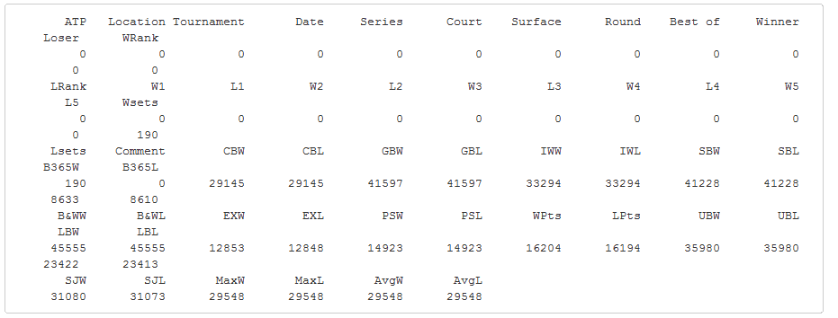
The data set contains 46,652 matches and 54 columns which is a decent amount of information to work with. Although there is quite a lot of features in the data set, I won’t be using all of them.

The table below gives a small peak at what the data looks like. It has some useful information like the Winner, Loser, Tournament and the Surface the games were played on.

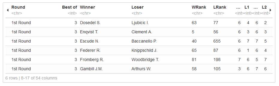
There are some missing values, so it’s a good idea to check which columns have missing values and calculate the frequency. There are missing values in the columns W1 – L5, which is understandable as not every match ends in 5 sets. The remaining columns are related to the betting odds.

Analysis

The first analysis I want to do is look at the top 20 players and compare their win rate over the years. This can be achieved by aggregating each player by year and surface and then counting how many wins and losses they had in each season.

The first data visualization I want to create in GGPlot is a heat map which shows the win percentage for the top 20 players based on the surface.

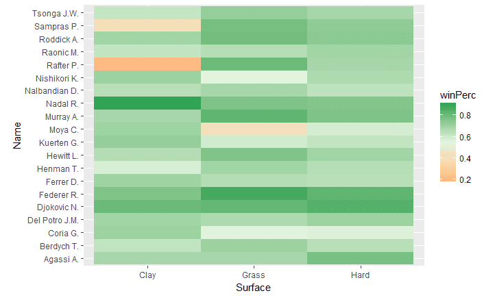
The heat map shows each player's win percentage, which is indicated by the intensity of the color. You can see that Nadal has an exceptional win rate on Clay. This is no surprise considering he is called the “King of Clay”.

Although having an overall high win rate is considered impressive, the main focus of players is to win at the major tournaments.

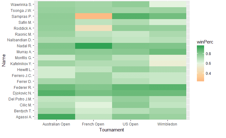
You can clearly see that Andre Agassi performed the best at the Australian Open. Pete Sampras had completely opposite results when competing in the French Open (low win rate) versus the US Open (higher win rate).

The next visualization is focused on looking at the win rate trend of the top 10 players over the years.

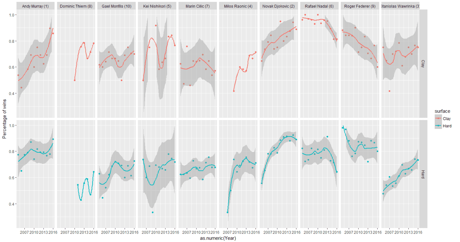
We can produce a plot which shows each player and how they compare over time. Some interesting trends include Novak Djokovic has shown consistent improved both in Clay and Hard court. Rafael Nadal has had the highest win rate for a season on Clay and Roger Federer is the same for Hard Courts. The most volatile when it comes to performance is Kei Nishikori, which shows that he has large troughs and peaks.

Summary

In summary, I used the R package GGPlot2 to produce some visualizations which highlighted some interesting insights about tennis players. I have only scratched the surface with some simple graphical analysis. I think there is a lot of space for modeling as well, that is, creating a model that can predict the winning records of a player.